Neuroscience

Neuroscience is a field with extraordinary potential, promising to catalyze fundamental scientific breakthroughs and to alleviate humanity of some of its worst medical afflictions. Neuroscientists study the structure, function, development and failure modes of the nervous system\(-\)the body’s electrical infrastructure\(-\)in hopes of answering questions related to disease, consciousness, and intelligence, both biological and artificial [1, 2, 3]. While the digital communication and information revolutions of the \(20\)^th century were driven primary by advancements in microelectronics [4], the technology of tomorrow may well be dominated by the union of brain and machine. The great futurist Ray Kurzweil predicts that by the \(2030\)s nanomachines will be inserted into human brains, allowing for enhanced cognitive and sensory bandwidth [5], and companies like Neuralink have already set out on that journey [6]. A maturation of brain science would be a decisive victory for all conscious creatures (if not for our intellectual enlightenment, for our health), so it deserves recognition and attention.

Sentience is likely the sum of an organism’s neuronal activity. Your brain contains \(\sim86\) billion neurons, and each one generates electrical signals called action potentials to communicate with its many neighbors [7]. The action potential is a critical event\(-\)it is the fundamental mode of information transmission and reception occurring in neural circuits. Communication between neurons is rooted in the action potential, and the aggregate action potential activity in a human brain yields emergent phenomena like thoughts and behavior.

Since its discovery in 1865 [8], the action potential has remained a central theme in neuroscience. However, despite the development of various scientific models that describe neural signaling [9], the underlying dynamics of action potentials are still not fully understood! Of the many competing models, I’d like to highlight one that hits home for me\(-\)the soliton hypothesis [10]. In this model, neural action potentials are treated as solitons, which are waveforms that exhibit unique stability due to a balance between dispersive and nonlinear effects. Solitons appear in various physical systems including Bose-Einstein condensates [11], black holes [12], the atmosphere [13] and, my favorite, nonlinear optics [11, 14, 15]. Propagation of light in nonlinear optical materials can manifest in a Light Bullet, which is the optical version of a soliton [11, 14, 15]. And therein lies my motivation for this article: I aim to convey the surprising physical similarities shared between optical solitons and the solitons that might occur in neural systems. But first, a cursory overview of basic neuronal structure and function.

Although there are many types of neurons [16], the following structural and functional description is generally true throughout the nervous system. Neurons function as biological information processing and memory units, and they serve to relay information throughout an organism. Like all cells, neurons contain a cell body, called the soma. The soma is responsible for the integration of incoming information, which it receives in the form of electrochemical signals. The signals, called action potentials, are detected by the soma’s tree-like extensions called dendrites. Action potentials originate at the somas of other neurons, and signal propagation occurs along the cell's axon, which extends off the soma and connects to (innervates) the dendrites of other neurons. The junctions formed between axons and dendrites are called synapses. Once an action potential terminates near the synapse, the axon terminal releases chemicals called neurotransmitters, which travel across the synaptic gap to the dendrites of an adjacent neuron and either excite, inhibit, or modulate the dendritic response. This enables the soma to gather information in the form of an analog signal, which in turn can induce the stimulated cell to fire an action potential down its own axon in an all-or-none response\(-\)a digital signal [17]. Many neurons together form neural circuits functioning as decision networks, giving rise to various higher-order processes like thoughts and behavior. Figure 1 shows the important elements of a typical neuron.

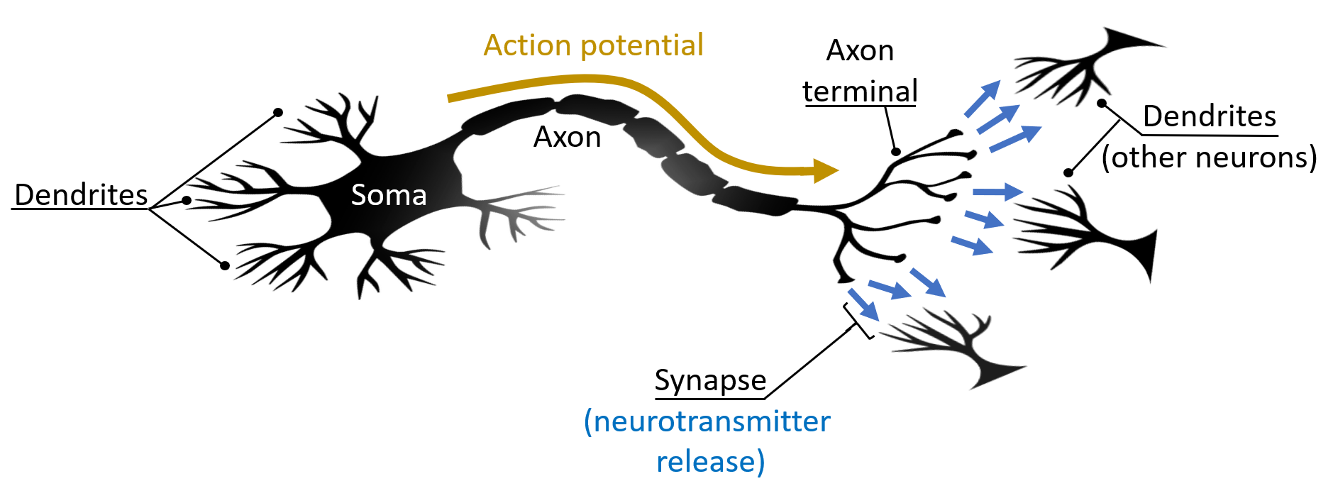
Figure 1: The structure of a typical neuron is shown here. The cell body, or soma, processes information that has been gathered by its dendrites. Under certain conditions, the soma can fire off an electrochemical signal called an action potential, which propagates down the neuron's axon and terminates near the axon terminal. Neurotransmitters are released at the synapse and picked up by dendrites of networked neurons.

Now for a deeper dive into neuronal signal transmission \(-\) the action potential.

One might guess that the electric signal transmitted down an axon is akin the conduction of current across a metallic wire. In a way, yes, both a wire and a neuron transmit electrical information due to the flow of charged particles. However, the mechanisms are completely different. Attach a metallic wire to the terminals of a voltage source, and an electric field is produced, which imparts a force on the weakly-bound electrons of the metal. The result? Electrons rush from one end of the wire to the other, producing electrical current. Electrical signal transmission along an axon is more complicated.

Like all other cells, neurons are enclosed by a membrane (\(\sim5\) nm in thickness [18]) that separates the internal cellular components from the extracellular environment. The membrane is comprised of a Phospholipid bilayer with embedded proteins that function as pumps and channels (see Figure 2). In addition to serving as a barrier, the membrane is a gateway that manages the flow of substances into and out of the cell\(-\)substances like waste products, essential nutrients and, crucially, ions. The regulation of ionic traffic establishes concentration gradients of ions across the membrane, and it is this essential feature that enables signal transmission along axons. Although several important ions contribute to neural signal propagation, the key players are Sodium (Na⁺) and Potassium (K⁺), so we'll focus on these.

A key regulator of ionic concentration gradients is the Sodium-Potassium pump. The pump is simply a protein embedded in the cell membrane (up to a tens of millions are found in each cell [19]) that actively transports K⁺ and Na⁺ across the membrane. For every 2 K⁺ moved into the cell, 3 Na⁺ are sent out. Furthermore, the membrane itself is somewhat more permeable to K⁺ than it is to Na⁺, which, along with the pump, dictates the equilibrium state of the ionic concentrations across the membrane. At equilibrium (no action signal transmission occurring), there is alot of K⁺ inside the cell, and alot of Na⁺ outside of it.

Crucially, in the equilibrium state the extracellular space is more positively charged than the cell's internal environment. The important consequence: an electrical potential difference exists across the membrane. Place a pair of electrodes across the membrane of a neuron in equilibrium, and you will measure a finite voltage called the resting potential: \(\Delta V_r \sim -70\) mV [16]. The negative sign just signifies that the cell's interior is more negative the environment. That's a very important property: a neuron in its equilibrium state will exhibit an electrical polarization across its membrane .

In addition to the pump, there are ion channels embedded in the membrane that selectively allow K⁺ or Na⁺ to flow down their concentration gradients. At equilibrium (\(\Delta V_r \sim -70\) mV) those channels are closed, but if some event (e.g., changes in pressure, temperature, light, sound, or signaling from other neurons) drives the membrane potential above a threshold value of \(\Delta V_t \sim -55\) mV [20], then the signaling process unfolds. First, Na⁺ channels open up, enabling Na⁺ to flow down its concentration gradient into the cell. The influx of positively charged Na⁺ pushes the membrane potential in the positive direction, peaking out at \(\Delta V_p \sim 10\) mV. When this happens, the polarization across the membrane is much lower in magnitude compared to its resting state, so we say that the membrane has depolarized. A few milliseconds later the Na⁺ channels close and K⁺ channels begin to open, resulting in a rapid movement of K⁺ into the extracellular space (down its concentration gradient). The potential difference across the membrane is driven towards large negative values, which overshoot the resting membrane potential, yielding a hyperpolarized potential of \(\Delta V_h \sim -75\) mV [20]. Finally, the K⁺ channels close, and the Sodium-Potassium pump restores the membrane potential to its equilibrium value. Figure 2 illustrates this sequence of events.

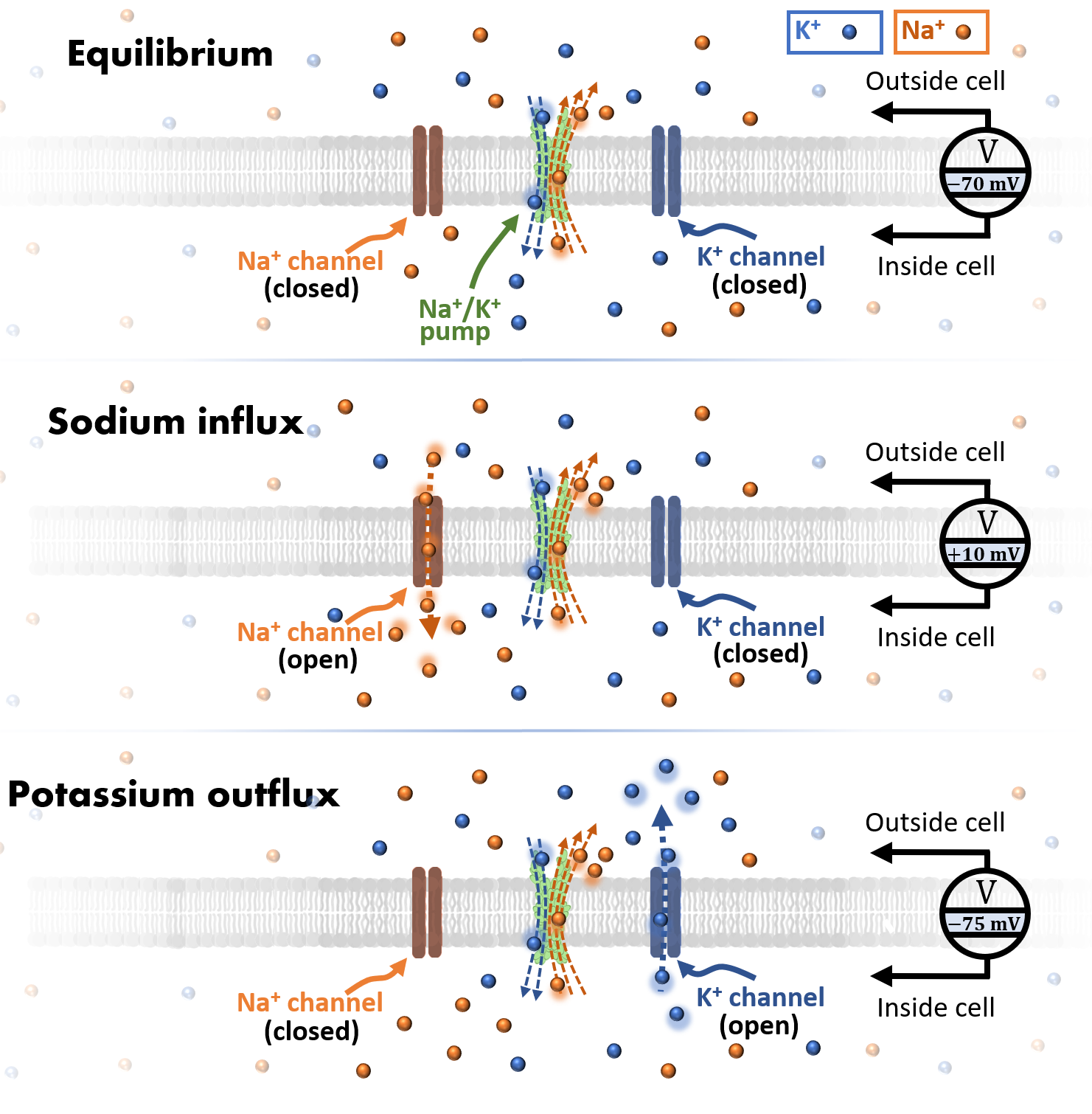
Figure 2: The stages of ion transport during action potential propagation are shown here. At equilibrium, the Sodium-Potassium pump actively moves K⁺ into and Na⁺ out of the cell. A large negative equilibrium (resting) potential is maintained. If a stimulus drives the potential above a threshold value, then Na⁺ channels will open, generating an influx of Na⁺ ions and a small positive membrane potential. Milliseconds later, Na⁺ channels close and K⁺ channels open, causing an outflux of K⁺ and a large negative potential across the membrane.

Great, so certain ions can flow into and out of the cell in response to a perturbation in voltage across the membrane. But how does that result in the propagation of a signal along an axon? Well, the description above considers a localized membrane region that has been driven to a potential above its threshold value (\(\Delta V_t \sim \)\(-55\) mV). The resultant influx of Na⁺ drives up the membrane potential further, but that increase in potential is somewhat delocalized. In addition to transport across the membrane, the ingoing Na⁺ diffuses along the membrane surface, increasing the potential over an extended range. The result? Adjacent Na⁺ ion channels open, catalyzing the ion transport events described above along a new slab of membrane. And so it goes, in a domino-like manner along the length of the axon until the signal reaches the axon terminal. Furthermore, the signal moves mainly in one direction, which occurs because hyperpolarized sections of membrane are temporarily inactive. Neuroscientists call this interval of inactivity the refractory period. For fans of electronics, that's diode-like behavior.

Qualitatively, this story captures all the important events that enable action potential propagation in neurons. Now lets take a more quantitative look at the dynamics.

The Hodgkin-Huxley (HH) Model is a powerful mathematical description of action potential propagation which was first introduced in 1952, leading to the 1963 Nobel Prize in Physiology or Medicine [9]. Despite having minimal insight into important molecular mechanisms regarding the regulation of ion permeability, Alan Hodgkin and Andrew Huxley used their model to successfully calculate various features of the action potential in giant squids. Along with an accurate prediction of the temporal shape of the electrical signal, the HH model was used to calculate the conduction velocity of the action potential to an accuracy of \(\sim\)10% (about 20 m/s) [9]. It was this quantitative precision that fortified the scientific prowess of the model.

The HH model makes a few simplifying assumptions. (1) The membrane can be described in terms of a capacitance \(C_m\). This should make sense, since there is a charge differential across the membrane, and fundamentally a capacitor stores separated charges. From simple capacitor logic, we can imagine a charge \(Q=C_mV_m\) stored by the membrane, where \(V_m\) is the membrane potential. (2) the Na⁺ and K⁺ ion channels can be regarded as resistors with time and voltage-dependent conductance \(G_{NA}\) and \(G_{K}\), respectively (conductance is just the inverse of resistance, \(G=1/R\)). This should also make sense: when activated, the ion channels allow for a certain amount ion flow, resulting in an ionic current across the channels \(I_i\). We can calculate this current if the conductance \(G\) is known for each channel, simply by invoking Ohm's Law: \(I_i = V_mG\). Additionally, the model accounts for "leak channels" that are always open and yield a current \(I_L\), which allows us to address the inherent partial permeability of the membrane to Na⁺ and K⁺. Note that a capacitive current can also be calculated, simply by taking the time derivative of the charge stored by the capacitive membrane: \(I_c = \frac{dQ}{dt} = C_m\frac{dV_m}{dt}\). So a temporal variation in the voltage across the membrane yields a capacitive current. The total current is just the sum of the capacitive current and the ionic current: \begin{equation} I = C_m\frac{dV_m}{dt} + \sum_i G_i\Delta V_i \tag{1} \end{equation} Here the sum over \(i\) accounts for current contributions due to each ion channel (Na⁺, K⁺ and leak channels). For each channel, we consdier the conductance \(G_i\) and the driving potential \(\Delta V_i = V_m - \Phi_i\), where \(\Phi_i\) is the Nernst equilibrium potential for each ion, which accounts for the interplay of forces on ions due to charge and consentration gradients. Figure 3 shows the simple circuit diagram encapsulated by Equation 1.

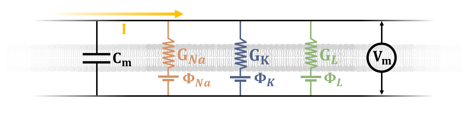
Figure 3: The circuit diagram shown here is the basis of the Hodgkin-Huxley model. Electrical elements are labeled, representing the cell membrane as a capacitor with capacitance \(C_m\), and Na⁺, K⁺ and leak channels as resistors with conductance \(G_{Na}\), \(G_{K}\) and \(G_{L}\), respectively. The Nernst equilibrium potentials for each channel are shown as voltage sources, labeled \(\Phi_{Na}\), \(\Phi_{K}\) and \(\Phi_{L}\), and the potential difference across the membrane is \(V_{m}\). A current \(I\) flows along the membrane due to the opening and closing of ion channels.

Although Equation 1 captures most of the dynamics of ion transport, the complete HH model requires a bit of parameter tuning based on empirical data. For the model to closely approximate experimentally-measured currents, three time and voltage-dependent variables (\(n, m\) and \(h\)) are incorporated into Equation 1, acting to appropriately gate the contributions of Na⁺ and K⁺ currents. The values of these gating parameters, along with the intermembrane voltages and currents, are fully summarized using four ordinary differential equations, including Equation 1. Iteratively solving these four coupled equations allows us to predict the time evolution of the action potential with remarkable accuracy! However, there is still substantial room for improvement. The dynamical description presented above has only considered Na⁺ and K⁺ ion channels, and their properties are quantified in a rather crude manner. Modern molecular genetics has revealed \(\sim 40\) genetic subunits acting to diversify the electrochemical properties of K⁺ channels alone, not to mention the various types and clustering behavior of Na⁺, Ca²⁺, and Cl^\(-\) channels [21]. More sophisticated models based on Hodgkin and Huxley's initial framework have been developed, with encouraging results [22, 23, 24], but many questions remain unanswered. To fully capture the physics of neural signaling, it might be time for a paradigm shift in our thought process of action potential dynamics.

Among the various competing models for neural action potential propagation is the soliton model, which describes the action potential as an electromechanical pulse exhibiting soliton-like dynamics. Let's unpack each of these characteristics.

First, unlike the HH model, the soliton model stresses the importance of mechanical effects during the action potential. This means that it's important to incorporate any structural changes occurring in the cell membrane as the electrical signal propagates. Intuitively, we should expect mechanical changes in the membrane, since the opening and closing of ion channels necessarily involves structural reorganization. However, instead of considering the ion channels directly, our new model focuses on the mechanics of the Phospholipid bilayer. Phospholipids are the macromolecules that make up the cell membrane, and they're comprised of Phosphate-based 'heads' and Carbon-chained 'tails'. At an organism's body temperature, the consistency of the Phospholipid membrane is fluid-like\(-\)that is, the molecules can move along the \(2\)-dimensional plane of the membrane with little resistance, in a type of random walk [25]. If the temperature falls to a low enough value, below the 'melting point' of the membrane, then Phospholipids become more rigid and the Carbon chains elongate due to trans isomerization, which is just a rotation of Carbon bonds to a particular configuration. This change in mechanical character to a more gel-like material is regarded as a type of phase transition, and it is shown in Figure 4.

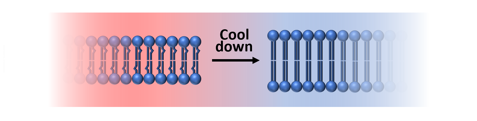
Figure 4: The Phospholipid bilayer is shown here in two phases. Above the melting point (higher temperatures), the membrane is fluid, with short tails containing kinks in the Carbon chains. Below the melting point, Phospholipids become more rigid and elongated, with a gel-like consistency.

Now for a crucial observation. As the action potential propagates, the membrane exhibits temperature fluctuations coincident with the electrical pulse. When ion channels first begin to open at a particular slab of membrane, the local temperature increases. Shortly thereafter, there is a measurable reduction in temperature [26]. And we know that the membrane undergoes structural changes in response to a temperature variation. So, we can think of the action potential as a temperature-dependent mechanical disturbance propagating along the membrane! Figure 5 serves as a visual aid for the process.

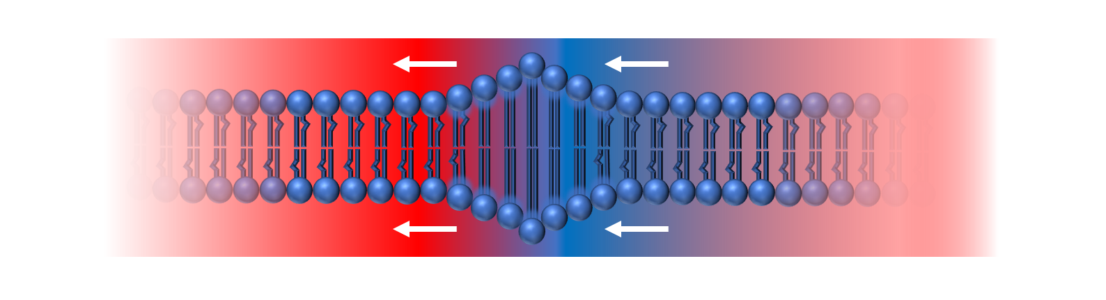
Figure 5: The Phospholipid bilayer will dynamically respond to temperature fluctuations during the action potential. As temperatures change from high (red) to low (blue), the membrane becomes more rigid and elongated, producing a thermally-induced mechanical perturbation that travels as a pulse along the membrane.

It's useful to think of the mechanical wave in terms of membrane density. Since molecules stretch and contract in response to the thermal agitation, the waveform can be quantified by the membrane density variation \(\Delta \rho\)\(-\)this might ring a bell if you're familiar with acoustics, as it basically describes a sound wave. Localized compression waves propagating through isolated neurons are well documented [27, 28], providing an empirical basis for this concept.

Ok, but what about the electrical information? Well, embedded in the membrane are various charged and polar substances, including the Phospholipids themselves! Thus, the sound wave naturally invokes an electrical response. So we have a mechanical wave propagating down the membrane, which is coupled to and electrical disturbance. This electromechanical wave is our action potential.

Now onto the soliton-like nature of the action potential. For some perspective, lets consider the first documented observation of soliton waves. John S. Russell, a Scottish naval architect, was the first to report on solitary waveforms in 1834 [29]:

"I believe I shall best introduce the phenomenon by describing the circumstances of my first acquaintance with it. I was observing the motion of a boat which was rapidly drawn along a narrow channel by a pair of horses, when the boat suddenly stopped\(-\)not so the mass of water in the channel which it had put in motion; it accumulated round the prow of the vessel in a state of violent agitation, then suddenly leaving it behind, rolled forward with great velocity, assuming the form of a large solitary elevation, a rounded, smooth and well-defined heap of water, which continued its course along the channel apparently without change of form or diminution of speed. I followed it on horseback, and overtook it still rolling on at a rate of some eight or nine miles an hour, preserving its original figure some thirty feet long and a foot to a foot and a half in height. Its height gradually diminished, and after a chase of one or two miles I lost it in the windings of the channel. Such, in the month of August 1834, was my first chance interview with that singular and beautiful phenomenon which I have called the Wave of Translation."

The solitary Wave of Translation described by Russell has since been referred to as a soliton, and his key insight\(-\)that the solitary wave propagates without changing its form over long distances\(-\)holds true for solitons in their various natural forms. More technically, solitons are waveforms that retain their shape during propagation due to a balance between nonlinear and dispersive effects. These terms stem from their roles in dispersive nonlinear partial differential equations, which constitute a class of equations describing a broad range of physical systems. In each system, the waveform can be described in terms of an amplitude \(A\) and frequency \(\omega_0\), which is the central value within a frequency band \(\Delta\omega\) that makes up the waveform.

By nonlinear, we mean that the magnitude of \(A\) influences the evolution of the waveform. For example, the velocity of the wave might be reduced at larger values of \(A\). And since the waveform is a pulse, the amplitude profile is described by a function that decays in magnitude away from its center (think Gaussian or hyperbolic secant). Thus, the central (highest amplitude) part of the waveform will travel at a reduced velocity compared to the pulse at its outskirts, where the amplitude is lower.

By dispersive, we mean that the velocity of the wave depends on its frequency. Since the wave is comprised of a frequency band \(\Delta\omega\), we can designate a unique velocity to each frequency component. Thus, we expect the waveform to change shape during propagation, since some frequencies will outpace others, resulting in either a spread or compression of the pulse in time. Just how these dynamics unfold depends on the initial distribution of frequencies and the shape of the dispersive curve for the frequency band comprising the pulse. For example, it might be the case that lower frequencies travel faster than higher ones\(-\)in optics, this is called normal dispersion. On the other hand, if higher frequencies outpace lower frequencies, the dispersion regime is anomalous. The specific shape of the dispersion function depends on the frequency band and the medium supporting the waveform.

Solitons can propagate if nonlinearities directly oppose the effects of dispersion. In the case of action potentials, It can formally be proven that in conditions where the membrane is undergoing a phase transition (between fluid and more rigid gel-like phases), a highly nonlinear dependence of the propagation velocity on membrane density arises [10]. This nonlinear propagation regime enables the density-dependence of the velocity to precisely counteract its frequency-dependence, and a stable waveform can propagate without changing its shape! The equation governing the propagation of the density wave in an axon membrane is of the following form [10]: \begin{equation} \frac{\partial^2 \Delta\rho}{\partial t^2} = \frac{\partial}{\partial z}(N\frac{\partial \Delta\rho}{\partial z}) + a\frac{\partial^4 \Delta\rho}{\partial z^4} \tag{2} \end{equation} Here \(\Delta\rho\) describes the magnitude of the local density variation constituting the neural pulse (serving the role of the soliton amplitude), \(t\) is time, and \(z\) is the direction of propagation. The first and second terms on the right-hand side represent the contribution of nonlinear and dispersive effects, respectively. The term \(N\) is a factor that determines the speed of sound (and hence the speed of the action potential) along the membrane, which has a nonlinear dependence on the density: \(N=N(\Delta\rho^m)\), where \(m>0\). The factor \(a\) determines the frequency dependence of the sound velocity. For soliton propagation to occur it must be true that \(a<0\), which results in higher frequencies propagating faster than lower ones. Near the phase transition of the membrane during the action potential, this condition is satisfied, and Equation 3 predicts the propagation of a stable solitary pulse with very little variation in its shape during transit. The fine balance is fundamentally a result of the thermodynamic influence of the phase transition on the velocity of sound, giving rise to the requisite density and frequency dependence [30, 31, 32, 33]

And that sums it up. But what is the utility of the soliton model? For one, it's an accurate framework for describing thermal and mechanical dynamics during action potential propagation, including changes in membrane thickness [34], length [27], and the reversible generation of heat [26]. Furthermore, the soliton model is an effective approach for predicting the influence of anesthetics on neuron signaling [35]. Although there are some drawbacks compared to more fully-developed frameworks based on Hodgkin and Huxley's seminal work, the soliton model is a powerful tool that might one day be unified with more traditional methods. For example, although the effects of ion channels are not explicitly accounted for, the soliton model does predict transmembrane currents that resemble those associated with ion channels [36].

So the quest for a complete description of neural dynamics is ongoing, and the path forward will surely consist of a series of paradigm shifts in the way we think about the physics of the brain. The soliton model might serve as one of many such paradigm shifts. And that shift is in a direction occupied by many fields, nonlinear optics being one of them. To close the topic, let's consider the similarities between the proposed solitons in nervous systems and those occurring during high-intensity light matter interactions.

At this point it's useful to skim through my primer on nonlinear optics, which describes the physics of high-intensity light-matter interactions. In short, modern ultrafast laser systems enable the generation of laser pulses with durations on the order of femtoseconds (\(1\) fs \(= 10\)^\(-15\) s). Due to their ultrashort durations, the optical powers and intensities of such laser pulses are very high. Thus, the electric fields that comprise an ultrashort pulse are extreme, and they tend to strongly perturb the materials that they interact with. Electrons are rapidly accelerated in the strong field, and some of them are even ripped away completely from their mother ions, producing a sea of free electrons called a plasma. This all manifests in a nonlinear light-matter interaction, meaning that the evolution of the pulse's electric field is highly sensitive to the field strength. And, just like neuronal action potential propagation, we can use a nonlinear partial differential equation to model the evolution of a powerful optical pulse. The gold standard in nonlinear optics is the Nonlinear Schrödinger equation, which takes the following form [37]: \begin{equation} \frac{\partial E}{\partial z}=iNE + ia\frac{\partial^2 E}{\partial t^2} + ib\nabla_\perp^2E \tag{3} \end{equation} Here \(E\) is the electric field amplitude, \(z\) is the propagation direction of the pulse, \(t\) is time, \(i\) is the imaginary unit, and \(\nabla_\perp^2 = \frac{\partial^2}{\partial x^2}+\frac{\partial^2}{\partial y^2}\) is the transverse Laplacian differential operator, where \(x\) and \(y\) are the directions that make up the plane containing the cross-sectional profile of the pulse. The first, second and third terms on the right-hand side account for the effects of refractive index modulations, dispersion (spreading of the pulse in time) and diffraction (spreading of the pulse in space), respectively. Here the parameter \(N\) captures the effects of the intensity-dependent refractive index (known as the Kerr effect) and effects due to plasma. The Kerr effect causes the beam to focus on its own, producing a smaller cross-sectional profile in space. On the other hand, plasma tends to defocus the beam. Both plasma and the Kerr effect also act to broaden the spectral bandwidth \(\Delta \omega\) of the pulse, which shortens the pulse duration. Furthermore, these two effects generate a time-dependent propagation velocity (high-intensity regions of the pulse travel slow, and regions with high plasma density speed up). The parameter \(a\) describes the dispersion regime: if \(a<0\), then the medium is normally-dispersive (so low frequencies outpace higher ones), otherwise the medium is anomalously dispersive (high frequencies travel faster than low ones). Finally, \(b\) is a parameter that is always positive, which ensures that diffraction acts to diverge the beam in the \(x-y\) plane.

Comparing Equation 3 for optical pulses to Equation 2 for neural pulses, we can immediately identify a few similarities. In both cases, we are modelling the evolution of an amplitude term\(-\)for neural pulses, it is the density variation \(\Delta\rho\), and in the optical regime it is the electric field amplitude \(E\). Dispersive and nonlinear effects influence the space-time evolution of each waveform. For optical pulses, there is an additional term describing diffraction, but mathematically the form is similar to dispersion\(-\)both effects are modelled simply differentiating (up to a few orders) in some dimension(s), which determines the nature of the pulse spreading. In each case, the amplitude determines the degree of nonlinearity, which is captured in the term \(N\). Both optical and neural pulses exhibit amplitude-sensitive propagation velocities, each varying with respect a baseline speed of light or speed of sound, respectively. And, just like neural pulses, optical pulses propagating under certain conditions will exhibit solitary wave behavior.

How do optical solitons form? Well, there are actually two types of solitons that can be generated during the nonlinear propagation of an optical pulse. (1) A temporal soliton is a pulse that does not spread in time during propagation. You can also think of this as sustained spatial confinement along the axis of propagation (\(z\) axis). Temporal solitons are generated when the nonlinear intensity/plasma-dependent refractive index modulates the phase of the beam (self-phase modulation) to counteract the effects of dispersion. In particular, self-phase modulation acts to produce light at lower and higher frequencies (with respect to the central frequency) near the front and back edges the pulse, respectively. When this happens in anomalously-dispersive materials, the high-frequency light generated at the trailing edge is swept forward, and low-frequency light is swept back. In this way, the slowing down of light near the front of the pulse allows the faster light at the back to "catch up", and the process occurs continuously, as long as the intensity is sufficiently high and the dispersion is anomalous. The result? A sustained temporal profile! A temporal soliton is born. (2) A spatial soliton is a pulse that does not spread in the \(x-y\) plane during propagation. A sustained spatial profile forms when self-focusing precisely counteracts the effects of diffraction and plasma-induced defocusing. And when the waveform exhibits both spatial and temporal solitary wave behavior? In that case, the pulse is a spatiotemporal soliton, commonly referred to as a Light Bullet [11, 14, 15]. Light Bullets represent a holy grain in nonlinear optics, and they have gained recent theoretical interest [38, 39, 15] owing to their physical novelty and scope of applications, which includes ultrafast digital logic [40] and high-fidelity data transmission that is free from restrictions imposed by conventional binary logic schemes [41].

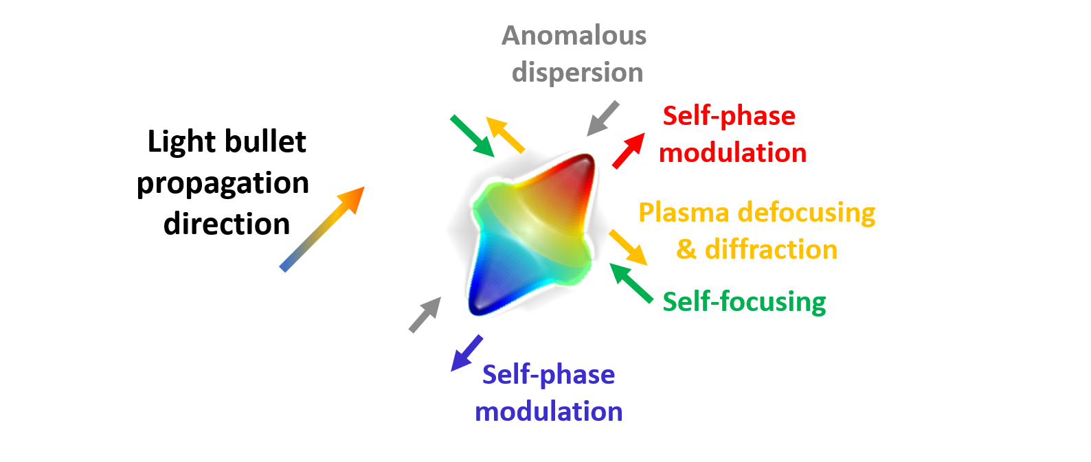
Figure 6: A Light Bullet is a spatio-temporally invariant pulse that forms due to a fine balance between various linear and nonlinear optical effects. Temporal confinement is achieved through nonlinear self-phase modulation counteracting the spreading of the pulse in anomalously-dispersive media. Spatial confinement occurs when nonlinear self-focusing balances the beam divergence due to plasma-induced defocusing and diffraction.

And there you have it, the Light Bullet in all its glory, described by mathematics that is strikingly similar to the novel soliton model developed by neuroscientists. The interdisciplinary nature of brain science may come as no surprise for its practitioners, but the gap between nonlinear optics and neuroscience is particularly wide, and its potential bridging by solitons should be noted carefully. If the analogy holds against rigorous empirical validation, the labors of each field will serve as untapped knowledge ripe for exchange, and with profound consequences.

Enjoying my content? Want to see an article on a different scientific topic? Help support my caffeine-driven creativity through Patreon! :)

[1] E. R. Kandel, Principles of Neural Science (McGraw-Hill Education, 2012).
[2] R. G. Shulman, Neuroscience: A Multidisciplinary, Multilevel Field. Brain Imaging: What it Can (and Cannot) Tell Us About Consciousness (Oxford University Press, 2013).
[3] A. H. Marblestone, G. Wayne, and K. P. Kording, "Toward an Integration of Deep Learning and Neuroscience", Front. Comput. Neurosc. 10, 94 (2016).
[4] J. D. Cressler, Silicon Earth: Introduction to Microelectronics and Nanotechnology (CRC Press, 2016).
[5] R. Kurzweil, The singularity is near: When humans transcend biology (New York: Viking, 2005).
[6] E. Musk, "An integrated brain-machine interface platform with thousands of channels", bioRxiv (2019).
[7] S. Herculano-Houzel, "The human brain in numbers: a linearly scaled-up primate brain", Front. Hum. Neurosci. 3, 31 (2009).
[8] S. M. Schuetze, "The discovery of the action potential", Trends Neurosci. 6, 164 (1983).
[9] A. L. Hodgkin and A. F. Huxley, " Currents carried by sodium and potassium ions through the membrane of the giant axon of Loligo ", J. Physiol. 116, 424 (1952).
[10] T. Heimburg and A. D. Jackson, "On soliton propagation in biomembranes and nerves", Proc. Natl. Acad. Sci. U.S.A. 102, 790 (2005).
[11] B. A. Malomed, D. Mihalache, F. Wise, and L. Torner, "Spatiotemporal optical solitons", J. Opt. B 7, R53 (2005).
[12] T. G. Philbin, C. Kuklewicz, S. Robertson, S. Hill, F. König, and U. Leonhardt, "Fiber-Optical Analog of the Event Horizon", Science 319, 1367 (2008).
[13] R. H. Clarke, R. K. Smith, and D. G. Reid, "The Morning Glory of the Gulf of Carpentaria: An Atmospheric Undular Bore", Mon. Weather Rev. 109, 1726 (1981).
[14] Y. Silberberg, "Collapse of optical pulses", Opt. Lett. 15, 1282 (1990).
[15] R. I. Grynko, G. C. Nagar, and B. Shim, "Wavelength-scaled laser filamentation in solids and plasma-assisted subcycle light-bullet generation in the long-wavelength infrared", Phys. Rev. A 98, 023844 (2018).
[16] T. H. Bullock, R. Orkand, and A. Grinnell, Introduction to nervous systems (WH Freeman, 1977).
[17] E. D. Adrian, "The all-or-none principle in nerve", J. Physiol. 47, 460 (1914).
[18] B. Alberts, A. Johnson, J. Lewis, M. Raff, K. Roberts, and P. Walter, Molecular Biology of the Cell (New York: Garland Science, 2002).
[19] M. Liang, J. Tian, L. Liu, S. Pierre , J. Liu, J. Shapiro, and Z. J. Xie, "Identification of a pool of non-pumping Na/K-ATPase", J. Biol. Chem 282, 10585 (2007).
[20] J. Seifter, A. Ratner, and D. Sloane, Concepts in Medical Physiology (Lippincott Williams & Wilkins, 2005).
[21] C. J. Schwiening, "A brief historical perspective: Hodgkin and Huxley", J Physiol. 590, 2571 (2012).
[22] M. D. Forrest, "Can the Thermodynamic Hodgkin–Huxley Model of Voltage-Dependent Conductance Extrapolate for Temperature?", Computation 2, 47 (2014).
[23] K. Pakdaman, M. Thieullen, and G. Wainrib, "Fluid limit theorems for stochastic hybrid systems with application to neuron models", Adv. Appl. Prob. 42, 761 (2010).
[24] Q. Zheng and G.-W. Wei, "Poisson–Boltzmann–Nernst–Planck model", J. Chem. Phys. 134, 194101 (2011).
[25] H. C. Berg, Random Walks in Biology (Princeton University Press, 1993).
[26] B. C. Abbott, A. V. Hill, and J. V. Howarth, "The positive and negative heat production associated with a nerve impulse", Proc. R. Soc. B 148, 149 (1958).
[27] E. Wilke and E. Atzler, "Experimentelle beiträge zum problem der reizleitung im nerven", Pflügers Arch. 146, 430 (1912).
[28] I. Tasaki, K. Kusano, and M. Byrne, "Rapid mechanical and thermal changes in the garfish olfactory nerve associated with a propagated impulse", Biophys. J. 55, 1033 (1989).
[29] J. S. Russell, Rep. Br. Assoc. Adv. Sci. 14th Meeting (1844).
[30] T. Heimburg, "Mechanical aspects of membrane thermodynamics. Estimation of the mechanical properties of lipid membranes close to the chain melting transition from calorimetry", Biochim. Biophys. Acta 1415, 147 (1998).
[31] H. Ebel, P. Grabitz, and T. Heimburg, "Enthalpy and volume changes in lipid membranes. I. The proportionality of heat and volume changes in the lipid melting transition and its implication for the elastic constants", J. Phys. Chem. B 105, 7353 (2001).
[32] W. Schrader, H. Ebel, P. Grabitz, E. Hanke, T. Heimburg, M. Hoeckel, M. Kahle, F. Wente, and U. Kaatze "Compressibility of lipid mixtures studied by calorimetry and ultrasonic velocity measurements", J. Phys. Chem. B 106, 6581 (2002).
[33] S. Mitaku and T. Date "Anomalies of nanosecond ultrasonic relaxation in the lipid bilayer transition", Biochim. Biophys. Acta 688, 411 (1982).
[34] K. Iwasa and I. Tasaki, "Mechanical changes in squid giant-axons associated with production of action potentials", Biochem. Biophys. Research Comm. 95, 1328 (1980).
[35] T. Heimburg and A. D. Jackson, "The thermodynamics of general anesthesia", Biophys. J. 92, 3159 (2007).
[36] T. Heimburg, "Lipid Ion Channels", Biophys. Chem. 150, 2 (2010).
[37] C. Sulem and P. L. Sulem, The Nonlinear Schrödinger Equation. Self-Focusing and Wave Collapse (Springer-Verlag, New York, 1999).
[38] P. Panagiotopoulos, P. Whalen, M. Kolesik, and J. V. Moloney, "Super high power mid-infrared femtosecond light bullet", Nat. Photon. 9, 543 (2015).
[39] C. Brée, I. Babushkin, U. Morgner, and A. Demircan, "Regularizing Aperiodic Cycles of Resonant Radiation in Filament Light Bullets", Phys. Rev. Lett. 118, 163901 (2017).
[40] R. Macleod, K. Wagner, and S. Blair, "(3+1)-dimensional optical soliton dragging logic", Phys. Rev. A 52, 3254 (1995).
[41] P. Rohrmann, A. Hause, and F. Mitschke, "Solitons beyond binary: possibility of fibre-optic transmission of two bits per clock period", Sci. Rep. 2, 866 (2012).