In layman's terms...
Light has been used in photography since the early \(1800\)s [1]. In its initial form, (analog) photography
relied on the exposure of light-sensitive chemicals to an image, which would be stored on a film.
Then came the digital revolution of the mid-\(1900\)s, which gave rise to semiconductor-based optoelectronic sensor arrays such as
charged-coupled device (CCD) and complementary metal-oxide semiconductor (CMOS) cameras. These devices are the
backbone of the many billions of cameras in use today [2]
, enabling us to take selfie photographs
on our smartphones, among the many other more productive camera-based activities. Crucially, all
photographic methods utilize the intensity patterns comprising the images we want to capture.
Holography, on the other hand, relies on a more fundamental property of light: the
electric
field
distribution [3]. This means that both the amplitude and phase of the light field are utilized.
With digital sensors, holograms can be captured at great speed and with high fidelity. Combine
this with advanced computational methods, and digital holograms can be used to reconstruct objects that
a typical intensity-based measurement is blind to, ranging from plasma columns to microscopic
biological structures. And it’s not just pretty pictures. Digital holography enables the acquisition
of quantitatively accurate data on the object's salient physical features. So, what’s the trick?
Fundamentals: the wave equation and its consequences
The basics of digital holography can be grasped with a firm understanding of light’s wavelike properties.
Classical electromagnetism provides that foundation by describing light as a wave comprised
of electric and magnetic fields, denoted by \(\boldsymbol{E}\) and \(\boldsymbol{B}\), respectively (bold font denotes
vector quantities, which have a magnitude and direction). Electromagnetic theory is
summarized succinctly using Maxwell’s four revolutionary equations [4]:
\begin{align}
\boldsymbol{\nabla} \cdot \boldsymbol{E} = \frac{\rho}{\epsilon_0} \tag{1}
\end{align}
\begin{align}
\boldsymbol{\nabla} \cdot \boldsymbol{B} = 0 \tag{2}
\end{align}
\begin{align}
\boldsymbol{\nabla} \times \boldsymbol{E} = -\frac{\partial \boldsymbol{B}}{\partial t} \tag{3}
\end{align}
\begin{align}
\boldsymbol{\nabla} \times \boldsymbol{B} = \mu_0\boldsymbol{J}+\mu_0\epsilon_0\frac{\partial \boldsymbol{E}}{\partial t} \tag{4}
\end{align}
Although some knowledge of vector calculus is useful for a deep appreciation of these equations,
we can proceed without dwelling on the mathematical subtleties. Briefly, \(\boldsymbol{\nabla}\) is the differential
gradient operator, \(\times\) is the cross product, and \(\cdot\) is the dot product.
Equation \((1)\) is Gauss's Law, which states that a charge density \(\rho\) (charge per unit volume)
is a source of an electric field
emanating outward from the charge (assuming \(\rho > 0\)). The parameter \(\epsilon_0\) is a
fundamental constant called the permittivity of free space. Equation \((2)\) is the analog of Gauss's law for
magnetism, which states that there are no magnetic monopoles (unlike electric charges, magnetic "charges"
always come in pairs: a bar magnet will always have two oppositely-oriented magnetic poles).
Equation \((3)\) is Faraday's law, which states that a magnetic field which varies over time \(t\) will induce
a time-varying electric field. Finally, equation \((4)\), called Ampere's Law, states that a magnetic field can be produced by either
a current density \(\boldsymbol{J}\) (flowing charges, confined to some volume) or a time-varying electric field. The parameter
\(\mu_0\) is a fundamental constant called the permeability of free space.
The remarkable consequence of these equations (in particular, the last two) is that
time-varying electric and magnetic
fields are inextricably coupled \(-\) the presence of a changing \(\boldsymbol{E}\) is always accompanied by a changing \(\boldsymbol{B}\)
!
Physically this manifests as a travelling wave of oscillating electric and magnetic fields: electromagnetic waves, also
known as light, radiation, and the beloved photon.
We can describe the propagation of electromagnetic waves by solving the wave equation, which can be established with
some simple manipulation of Maxwell's equations:
\begin{equation}
\nabla^2\boldsymbol{E} = \frac{1}{c^2}\frac{\partial^2 \boldsymbol{E}}{\partial t^2} \tag{5}
\end{equation}
This equation describes the spatial-temporal evolution of an electromagnetic wave in terms of its electric field (we
could just as well describe the wave using its magnetic field, but that would be redundant for our purposes).
The term \(c\) is the speed of light in vacuum, which
governs the universal speed limit for the transmission of information in our universe. In materials, the light field interacts
with charges (electrons) which wiggle in response to the field, causing them to generate their own electromagnetic waves.
The resultant waveform is a superposition of the incoming wave and wave that has been re-radiated by the wiggling charges,
and that resultant field travels at a reduced speed \(v = \frac{c}{n}\), where the term \(n\) is the refractive index of
the material. When propagation occurs within a material, we can simply replace \(c\) with \(v\) in our wave equation.
The wave equation has many solutions, with the most simple being a plane electromagnetic wave:
\begin{equation}
\boldsymbol{E}(z,t) = \boldsymbol{E}_0\cos(kz - \omega t) \tag{6}
\end{equation}
For simplicity, we have assumed that the wave is travelling along the \(z\) direction. The electric field
amplitude is \(\boldsymbol{E}_0\) and the wavenumber is \(k = \frac{n\omega}{c}\),
where \(\omega\) is the angular frequency of the wave (the electric
and magnetic fields oscillate at the rate described by \(\omega\)).
The argument of the cosine, \(\Phi = kz - \omega t\),
is called the phase of the wave, which
describes the instantaneous oscillatory state of the fields. For example, if \(\Phi = 0\), then \(\boldsymbol{E}(z,t)\)
is maximized, whereas if \(\Phi = \frac{\pi}{2}\), then \(\boldsymbol{E}(z,t)\) is \(0\). Figure 1
shows a typical representation of the plane
wave solution: electric and magnetic fields oscillate in orthogonal directions (along \(x\) and \(y\), respectively), and
the field propagates along \(z\).
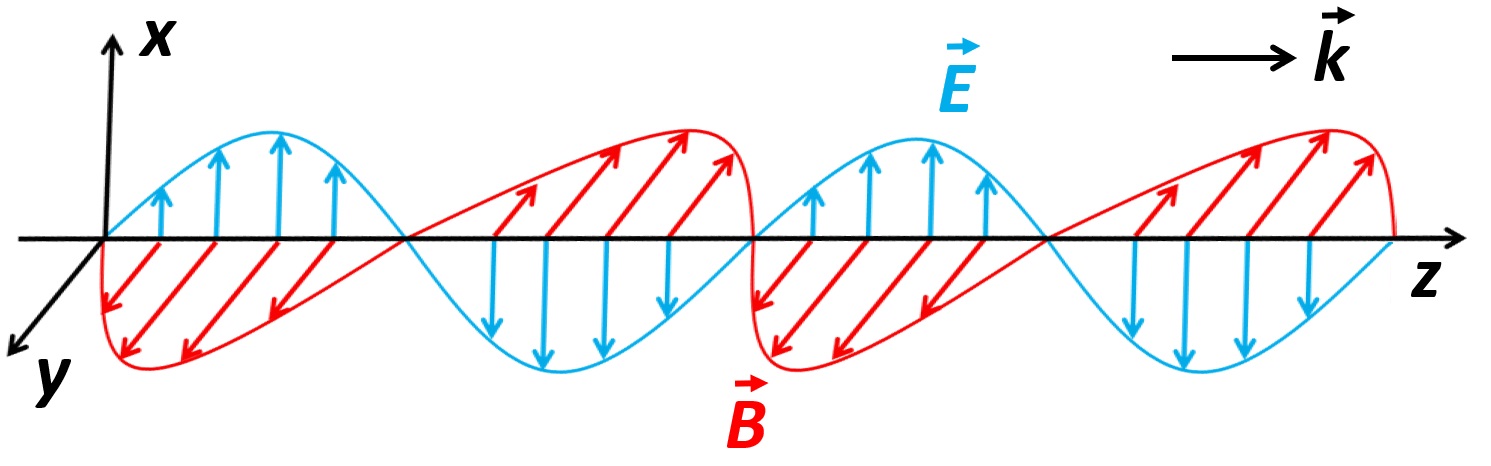
Figure 1: An electromagnetic wave consists of electric (blue) and magnetic (red) fields oscillating in space and time. The wave propagates in the \(z\) direction.
According to equation \((6)\) the ideal plane wave is
a series of infinite planes of constant field amplitude, but that's actually too much of an ideality for nature to support.
In reality, the amplitude will vary over \(x\) and \(y\)! For example, a typical laser beam's field amplitude
can be described using a Gaussian function: \(E_0(x,y) = E_{max}e^{[-\frac{x^2+y^2}{w_0^2}]}\) (note that I've
dropped the vector notation \(-\) let's just assume from now on that the electric field is along \(x\)). Here \(E_{max}\)
is the peak field amplitude (occurring at the center of the Gaussian) and
\(w_0\) is a characteristic radius (the position in space, relative to \(x = y = 0\), at which
the field amplitude falls to a value of \(E_0/e\), where \(e\) is Euler's number).
So, how does the electromagnetic wave evolve as it propagates? In particular, we're interested in how the spatial profile of the
wave behaves, since this is what we'll be utilizing for basic digital holography.
The beam's spatial evolution all depends on its initial spatial amplitude profile \(E_0(x,y)\), and
the initial spatial component of its phase \(\Phi_s(x,y) = \int \frac{n(x,y,z)\omega}{c}dz\) (note that instead of simple multiplication, we
have integrated over \(z\), which is required if the refractive index is varying in space).
In the simplest case, if the field amplitude and phase are Gaussian over \(x\) and \(y\), then the beam will simply spread in the \(x\) and \(y\)
directions as it propagates
along \(z\), becoming a larger Gaussian. Fundamentally, this is a result of diffraction: all beams spread during propagation
(unless if some focusing element is implemented). Figure 2
illustrates the evolution of a Gaussian beam with a central wavelength of \(\lambda = 800\) nm and an input diameter of
\(0.2\) cm. Propagation is modeled in air over a distance of \(20\) m, where the beam expands to a final
diameter of \(0.33\) cm.
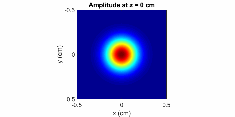
Figure 2: A beam with a Gaussian amplitude distribution simply spreads as it propagates. Here the wavelength is \(\lambda = 800\) nm, the initial beam diameter is \(0.33\) cm and the propagation distance is \(20\) m in air.
Great. So I numerically propagated the field.
How did I do that?
Well, I'm only interested in the evolution of the spatial mode, so
I ignore any time-dependent behavior (the \(\omega t\) component of the phase). Therefore, I seek a solution to a time-independent
version of the wave equation. I can describe the solution in terms of Fourier Transforms:
\begin{equation}
E(x,y;z)=\mathscr{F}_{xy}^{-1}\{\mathscr{F}_{xy}\{E_0(x,y)\}\mathscr{H}(z)\} \tag{7}
\end{equation}
Here \(E(x,y;z)\) is the electric field profile along coordinates \(x\) and \(y\) at some distance \(z\) from the
beginning of propagation. We have taken the Fourier Transform \(\mathscr{F}_{xy}\{\}\)
along the \(x-y\) plane of the input electric field \(E_0(x,y)\), and then multiplied it by
the function \(\mathscr{H}(z)\), which is called the spatial frequency transfer function. \(\mathscr{H}\)
is a wavelength-dependent quantity that describes the beam's evolution Fourier space, in terms of the spatial frequencies
\(\mu_x\) and \(\mu_y\) (these are conjugate Fourier variables of \(x\) and \(y\)). Finally, we perform an inverse Fourier
Transform \(\mathscr{F}_{xy}^{-1}\{\}\) of that product, which yields the field distribution in the \(x-y\) plane at \(z\)! This
numerical technique is called the Angular Spectrum Method, and it's a powerful tool for all sorts of computations in optical
physics and engineering [5].
To perform the computation, you can use any programming language with the fast Fourier Transform (FFT) functionality \(-\) I prefer MATLAB,
but there are many great options, like Python or C.
Note that the calculated \(E(x,y;z)\) is in general a complex number, enabling the simultaneous calculation of amplitude and phase. Expressing
The field in terms of imaginary and real parts, the complex number representation is:
\begin{equation}
E(x,y;z) = E_{RE}(x,y;z) + iE_{IM}(x,y;z) \tag{8}
\end{equation}
Here \(i\) is the imaginary unit (recall \(i^2=-1\)). To generate the beam profiles shown in Figure 2
I have calculated the amplitude according to \(A(x,y;z) = \sqrt{E_{RE}(x,y;z)^2 + E_{IM}(x,y;z)^2}\) \(-\) I did this in a step-wise
fashion to demonstrate the evolution of the beam over the course of propagation. I could just as easily have plotted the phase by computing
\(\Phi(x,y;z) = \tan^{-1}\{\frac{E_{IM}(x,y;z)}{E_{RE}(x,y;z)}\}\). Based on that calculation, a Gaussian phase front simply
spreads to a larger Gaussian during propagation, just like the amplitude.
A technical side note: I'm doing my modeling with a well-defined central wavelength \(\lambda\), assuming a monochromatic (single wavelength)
source. Typically such as source is a laser, which has the nice property of emitting coherent light, composed of wavefronts
with well-defined phase relationships. Coherence manifests pronounced diffractive effects, enabling the experimental
realization of digital holography. So keep in mind that we're assuming that a coherent laser light source is used.
Now let's add one more layer of complexity. Suppose there is some local variation in \(E_0(x,y)\), perhaps due to a small absorptive
material in the beam's path. How does the beam evolve when perturbed by that structure? To find out, let's propagate the field using the Angular
Spectrum Method, but this time set the initial field so that there is an amplitude minimum near the center of the Gaussian. I demonstrate this
in Figure 3: an input Gaussian beam has an amplitude dip at its center
in the shape of a circle with a \(\sim100\) μm diameter, and it propagates over a distance of \(40\) cm. For this case, I also plot
the evolution of the phase front, which is initially flat.
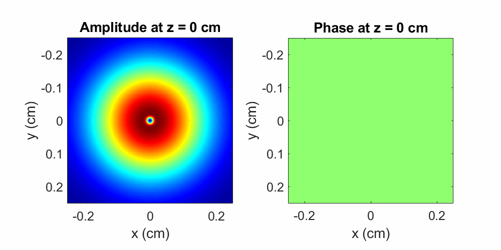
Figure 3: A Gaussian beam with a \(\sim100\times100\) μm2 amplitude dip propagates over a distance of \(40\) cm in air. The initial perturbation induces pronounced diffractive effects during propagation, as shown by the evolving amplitude oscillations. The phase front is initially flat, but ripples appear during propagation. Here the wavelength is \(\lambda = 800\) nm and the initial beam diameter is \(0.2\) cm.
After experiencing the amplitude perturbation, the beam's spatial evolution is drastically altered compared to the unperturbed case.
Instead of simply becoming a
larger Gaussian, a series of concentric rings (amplitude minima and maxima) emanate outward from the center of the beam! The spreading of these rings
resembles the behavior of water waves caused by a rock thrown into pond. A direct consequence of diffraction, this effect
illustrates the wavelike nature of light, which will always occur in the presence of some amplitude modulation. The magnitude, direction, and
rate of spreading of these oscillations depends directly on the perturbation shape and absorptive properties: (a) smaller objects will induce
more diffraction and (b) more absorptive objects will induce more diffraction. Taking a look at the phase front, note that although initially flat,
the phase profile exhibits oscillations during propagation! That is, the amplitude modulation has affected the evolution of the phase
front. A very important observation to keep in mind as we proceed.
So amplitude perturbations yield strong diffractive effects. What about phase perturbations? By phase perturbation, I mean that the object
which modulates the beam is transparent (it does not absorb any light) and propagation through the object changes the phase profile of the beam. Generally this happens
when the beam encounters a local (non-attenuating) refractive index change. A great example is a simple droplet of water, and a laser beam in the visible wavelength range.
A beam propagating through the droplet will see a refractive index \(n\) of \(1.33\), localized over a small region of the beam. If the surrounding medium is
air (with an index of \(1\)), then as the beam traverses the droplet, it acquires phase faster where the water is present due to a local index change of \(\Delta n = 0.33\).
Now we can assume that the amplitude profile is unaltered
(no absorption), and set the initial phase profile to have a small phase perturbation near the beam's center due to \(\Delta n\). Figure 4
shows the evolution of such a beam, having encountered a water droplet with dimensions \(100\times750\times400\) μm3.
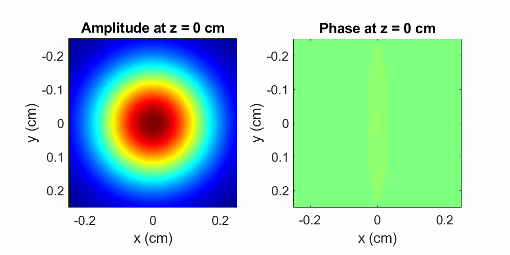
Figure 4: A Gaussian beam with a \(100\times750\) μm2 phase modulation propagates over a distance of \(40\) cm in air. The initial perturbation induces pronounced diffractive effects during propagation, as shown by the evolving amplitude and phase oscillations. Oscillations spread faster along the dimension where the phase object is smaller (along \(x\)). Here the wavelength is \(\lambda = 800\) nm and the initial beam diameter is \(0.2\) cm
As with the amplitude modulation, a beam with a perturbed phase profile will exhibit phase and amplitude ripples during propagation (again we observe that the amplitude and phase are co-dependent).
Additionally, since the water droplet is thinner along \(x\) than it is along \(y\), the diffractive effects shown in
Figure 4 are more pronounced diffractive along the \(x\) direction
(spatially-confined perturbations cause more diffraction), resulting in an asymmetrical spreading of the ripples.
So there you have it: a laser beam with some imperfection in its profile (an abrupt amplitude or phase variation) will exhibit diffractive
effects as it propagates. Instead
of the water droplet or the absorptive feature from the previous example, we can substitute a more complicated structure
that induces both phase and amplitude perturbations. And, regardless of how complex we make the perturbing structure, we will
always be able to accurately predict its effect on the wavefront using our propagation strategy! With this basic framework, we
can understand the principles of digital holography.
In-line digital holography: a lensless microscopy
Suppose we want to visualize some transparent object, such as a biological cell (perhaps a human egg cell, which is \(\sim100\) μm in diameter).
Let's assume that the cell is mostly water, constituting a local index change of \(\Delta n = 0.33\) relative to air. Our goal: measure the size
and shape of the cell with micron-level accuracy.
Now to appreciate how a simple photographic technique wouldn’t cut it here, let's think about what a digital sensor (or any photographic recording
medium) measures when recording a light pattern. The spatial distribution of the photons making up the field is captured by the sensor,
but that distribution is not a direct representation of the electric field in terms of amplitude and phase. Instead, the sensor captures
an intensity pattern. Formally, intensity is related to magnitude of the electric field amplitude squared:
\begin{equation}
I(x,y) \sim |A(x,y)|^2 \tag{9}
\end{equation}
Notice what's missing \(-\) the phase! So, our sensor can give us details about the amplitude (just
take the square root of the measured intensity profile), but the phase is lost. And remember, we're measuring
a transparent cell. So even if we use a lens to form an image of the object on our sensor, we'd simply
record the beam profile without any phase information. Not so useful for precise measurements of refractive
index modulations.
Enter digital holography, a lensless form of microscopy capable of quantitatively accurate phase (and amplitude)
object measurements. Let's consider the simplest variant of digital holography, called in-line holography,
which derives its name from the single beam used for the recording of holograms. I show
a simplified experimental setup in Figure 5.
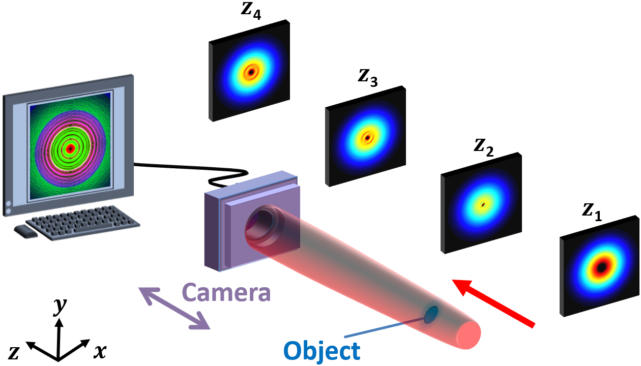
Figure 5: A simplified digital in-line holography experimental setup is shown here. A beam propagating along \(z\) traverses a sample, which induces diffraction, and a charge-coupled device (CCD) camera captures the diffraction pattern at a few locations along the propagation path.
To implement in-line holography, we simply need a laser beam and an array detector, such as a charge-coupled
device (CCD) camera. Now take the object of interest (our \(100\) μm thick egg cell) and send the beam
through it. We already know what will happen: although the cell is transparent, it's index difference \(\Delta n\)
compared to the surrounding air will impart a local change to the beam's phase front. And then, as expected, diffraction.
Now simply record the diffraction patterns using the camera at a few different locations along the beam's
propagation direction \(z\), and note those locations. And that's it! The rest is purely computational.
Note the simplicity of the experimental scheme I've described. Crucially, there isn't a single lens in
the setup I've shown! The implication? We are not imaging the object \(-\) we do not want to, and we cannot,
since it's transparent. The key here is that we're recording diffraction (interference) patterns. These are
holographic recordings!
So, all we have are diffraction patterns. How can we use them to gain useful information about our object? Well,
we can use our knowledge of beam propagation (see the previous section) to numerically reconstruct the object.
There are several algorithms that can be used for numerical reconstruction, but I'll describe the most straight-forward
one (in my opinion) called the Gerchberg-Saxton algorithm [6].
Referring to Figure 5, suppose that the object is located at plane
\(z_1\). Now consider the intensity recording at plane \(z_2\). There is no information about the phase in that data,
but the amplitude can be attained simply by taking the square root of the intensity profile: \(A_2(x,y) = \sqrt{I_2(x,y})\).
Great, so we can turn to our numerical propagation scheme and set the input field to be the amplitude at \(z_2\), leaving the
phase as some arbitrary flat profile.
Next, let's numerically propagate this field a distance \(\Delta z = z_3 - z_2\) to the \(z_3\) plane with the Angular Spectrum Method.
This allows us to calculate some electric field (both amplitude and phase) at \(z_3\). We can take that calculated field amplitude \(A_3\)
and compare it with the experimentally-measured amplitude at that plane, but we don't expect them to match. Why? Well, although
the amplitude at \(z_2\) was properly set, we ignored all features in the input phase, since that information was lacking! Thus, since the calculated amplitude
is not correct, we don't expect the phase to be correct either. Next, let's replace
the calculated amplitude at \(z_3\) with the experimentally measured amplitude, but leave the phase untouched.
Propagate to \(z_4\), and replace the calculated amplitude with experimental measurement, again leaving the phase untouched. Now that there are
no more experimental planes to compare with in the forward direction, we must propagate backward. No big deal \(-\) just propagate
back to \(z_2\) (which is very simple to compute, just make your \(\Delta z\) a negative quantity). Now repeat the procedure, and
for each step compare the calculated amplitude to the experimental data, without modifying phase. Eventually something wonderful happens:
convergence! After enough iterations, you will notice that the calculated amplitude very closely approximates the measured one. This will be true at all planes. Magic?
No. Along with the amplitude, the phase has converged, reaching a distribution approximating the experiment.
Now we can propagate to wherever we want and reproduce the experimental field at that location. Naturally, we choose to back-propagate
to the plane\(z_1\), where the object resides! I illustrate the important features of the algorithm in Figure 6.
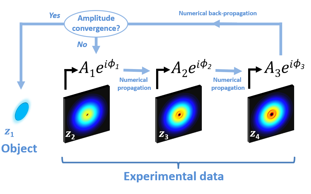
Figure 6: Numerical reconstruction algorithm using data taken using in-line holography for three diffraction planes. The amplitude of a data set is calculated by taking the square root of the measured intensity, and the beam is numerically propagated to the next plane. Calculated amplitudes are replaced with experimental distributions for each measurement location, followed by back-propagation to the first plane. If the calculated amplitude converges to the measurement, back propagation to the object plane is used to reconstruct the object. Otherwise, the algorithm is iteratively performed until convergence.
So we have calculated the electric field profile at the object plane. This is very useful, because it
gives us a great deal of information about the object's optical properties. In our example we have
considered a transparent egg cell, and we can use our reconstructed phase profile to extract the lateral
(\(x-y\)) profile of the cell. If the cell exhibits variation in its refractive index, we can extract that
information too, since it's all embedded in the phase profile. Furthermore, the absorptive properties of the
object are accessible too, since the amplitude at the object plane has been calculated.
Note that my experimental description of the in-line holography scheme is a highly simplified. As with conventional
(intensity-based) microscopy, the lateral resolution of digital holographic systems is limited by the
numerical aperture (\(NA\)) of the system. So, although no lens is required
for numerical reconstruction of the object, various additional optics are often implemented to improve the
resolving power of digital holography. Axially (along \(z\)), digital holography offers unprecedented
resolution capabilities, with reported accuracies as good as \(5\) nm
[7].
Furthermore, the in-line setup is only one of a variety of digital holographic schemes. Alternatives include
super resolution holography [8],
phase-shifting holography [9],
and Fourier holography [10],
among countless others [11].
Moreover, since the heart digital holography is computational, a rich variety of numerical methods can be utilized to improve the
reconstruction techniques, including the use of advanced deep learning algorithms for amplitude and phase reconstruction
[12].
Digital holography is a promising technology with a broad range of applications, including the monitoring
of fundamental biological processes like the cell cycle
[13],
dynamic measurements of micro electromechanical systems (MEMS) [14],
advanced flow cytometry [15],
optical voice encryption [16],
and various industrial inspection techniques [17].
One day holographic measurements might even play a role in the discovery of extraterrestrial life [18
,
19]!
Finally, if an ultrashort pulse is used to holographically probe a dynamically-evolving ultrafast event, then time-resolved
phase "movies" can be constructed, providing an intuitive visualization of exotic physical process as well
as important quantitative information such as refractive index modulations and instantaneous plasma densities
[20, 21, 22, 23, 24]
.
Digital holography has great potential for creative innovation both experimentally and computationally, and it
is likely to be a high-impact quantitative imaging modality for years to come.
References
[1]
R. Hirsch, Seizing the Light: A History of Photography (McGraw-Hill, 2018).
[2]
J. D. Cressler, Silicon Earth: Introduction to Microelectronics and Nanotechnology (CRC Press, 2016).
[3]
D. Gabor, "A New Microcscopic Principle", Nature 161, 777 (1948).
[4]
J. D. Jackson, Classical Electrodynamics (Wiley, 1975).
[5]
J. W. Goodman, Introduction to Fourier Optics (Roberts and Company Publishers, 2005).
[6]
R. W. Gerchberg and W. O. Saxton, "
A practical algorithm for the determination of the phase from image and
diffraction plane pictures
", Optik 35, 237 (1972).
[7]
B. Kemper, P. Langehanenberg, and G. Von Bally, "
Digital Holographic Microscopy:
A New Method for Surface Analysis and Marker‐Free Dynamic Life Cell Imaging
", Optik & Photonik 2, 41 (2007).
[8]
M. Paturzo, F. Merola, S. Grilli, S. De Nicola, A Finizio, and P. Ferraro, "
Super-resolution in digital holography
by a two-dimensional dynamic phase grating
", Opt. Express 16, 17107 (2008).
[9]
I. Yamaguchi and T. Zhang, "Phase-shifting digital holography", Opt. Lett. 22, 1268 (1997).
[10]
C. Wagner, S. Seebacher, W. Osten, and W. Juptner, "
Digital recording and numerical
reconstruction of lensless Fourier holograms in optical metrology
", Appl. Opt. 38, 4812 (1999).
[11]
M. K. Kim, Digital holographic microscopy (Springer, 2011).
[12]
Y. Rivenson, Y. Zhang, H. Günaydın, D. Teng, and A. Ozcan, "
Phase recovery and holographic image reconstruction
using deep learning in neural networks
", Light Sci. Appl. 7, 17141 (2018).
[13]
B. Rappaz, E. Cano, T. Colomb, J. Kühn, C. Depeursinge, V. Simanis, P. J. Magistretti, and
P. Marquet, "
Noninvasive characterization of the fission yeast cell cycle by monitoring dry mass with digital
holographic microscopy
", J. Biomed. Opt. 14, 034049 (2009).
[14]
E. Yves, N. Aspert, and F. Marquet, "
Dynamical Topography Measurements of MEMS up to 25 MHz, Through Transparent Window,
and in Liquid by Digital Holographic Microscope (DHM)
", AIP Conf. Proc. 1457, 71 (2012).
[15]
F. C. Cheong, B. Sun, R. Dreyfus, J. Amato-Grill, K. Xiao, L. Dixon, D. G. Grier,
"Flow visualization and flow cytometry with holographic video microscopy", Opt. Express 17, 13071 (2009).
[16]
S. K. Rajput and O. Matoba, "Optical voice encryption based on digital holography", Opt. Lett. 42,
4619 (2017).
[17]
E. Yves, E. Cuche, F. Marquet, N. Aspert, P. Marquet, J. Kühn, M. Botkine and T. Colomb,
"
Digital Holography Microscopy (DHM): Fast and robust systems for industrial inspection with
interferometer resolution
", Optical Measurement Systems for Industrial Inspection IV. 5856, 930 (2005).
[18]
E. Serabyn, K. Liewer, C. Lindensmith, K.Wallace, and J. Nadeau, "Compact, lensless digital holographic microscope for remote microbiology", Opt. Express 24,
28540 (2016).
[19]
E. Serabyn, K. Wallace, K. Liewer, C. Lindensmith, and J. Nadeau, "Digital holographic microscopy for remote life detection", Unconventional
Optical Imaging, 10677, 1067724 (2018).
[20]
M. Centurion, Y. Pu, and D. Psaltis, "Holographic capture of femtosecond pulse propagation", J. Appl. Phys. 100, 063104
(2006).
[21]
G. Rodriguez, A. R. Valenzuela, B. Yellampalle, M. J. Schmitt,
and K.-Y. Kim, "In-line holographic imaging and electron density extraction of ultrafast ionized air filaments", J. Opt. Soc. Am. B 25, 1988 (2008).
[22]
D. G. Papazoglou and S. Tzortzakis, "In-line holography for the characterization of ultrafast laser filamentation in transparent media", Appl. Phys. Lett. 93,
041120 (2008).
[23]
D. Abdollahpour, D. G. Papazoglou, and S. Tzortzakis, "Four-dimensional visualization of single and multiple laser filaments using in-line holographic microscopy", Phys.
Rev. A 84, 053809 (2011).
[24]
R. I. Grynko, D. L. Weerawarne, and B. Shim, "
Effects of higher-order nonlinear processes
on harmonic-generation phase matching
", Phys. Rev. A 96, 013816 (2017).
Try the interactive simulator
Holographic reconstruction depends on how a wavefront propagates after the object plane. Explore free-space Gaussian beam diffraction in real time using the Angular Spectrum Method — a physically exact Fourier-domain technique that works from the near field to the far field. Apply a thin lens or a phase object and watch the beam evolve interactively.
Launch Beam Diffraction Tool →